Bernoulli distribution & binomial trials

Bernoulli distribution

Bernoulli distribution contains categorical variables, and they are like qualitative attributes. It has only binary outcomes like success/failure, yes/no, like/dislike, etc.
With a Bernoulli random variable, we will have only one trial.

There is nothing in between to find a mean or something else.

Success = 1
Failure = 0

The mean is calculated using the probability-weighted sum.

µ = (probability of failure)*0 + (probability of success)*1

If the probability of success is p, then the likelihood of failure will be q = (1-p)

Mean = µ = E[X] = (1-p) * 0 + p * 1
= p

Variance = ν = σ² = E[(X-µ)²] = Σ(x-µ)²*p(x)
= (1-p)(0-p)² + p (1-p)²
= p² - p³ + p - 2p² + p³
= p(1-P) = pq

Standard deviation = σ = √(p(1-p)) = √(pq)

When the event is iid (identical independent distribution), then.

(iid: all samples are mutually independent & all samples will have the same probability distribution)

Variance of sample mean = ν’ = σ²/n

(Please read this article for details standard Error)

Standard error = Standard deviation of statistics
= SE = √ν’ = σ/√n

If the event is fair, then.

p = ½
σ = √(½ * ½) = ½
SE = 1/(2√n)

Example:

SE for a 15 coin flips, If each event is fair & iid

SE = 1/(2√15) = 0.1291 = 12.91%

A set of R commands will return the above value.

Generate 1000 rows of trials with each row contain 1500 individual trials  
trials <- matrix(sample(0:1, 15000, TRUE), 1000)

Find means of each row  
meanofrows <- apply(trials, 1, mean)

Find standard deviation of means  
sd(meanofrows) = 0.1266 = 12.66% (This is approximately equal to 12.91%)

Binomial trials

Binomial trials are generated from iid Bernoulli trials.

Let X₁, X₂, X₃ … X_n are iid bernoulli trials then

$\begin{array}{c} \text{The} \, \text{binomial} \, \text{random} \, \text{variable} \\ X = \sum_{i=1}^n X_{i} \\ \text{ Binomial} \, \text{mass} \, \text{function } \\ = P_{X=x} = \left( \begin{array}{c} n \\\\ x \end{array} \right) p^{x} (1-p)^{n-x} \\\\ \text{ Here} \, \text{read } \left( \begin{array}{c} n \\\\ x \end{array} \right) \text{ as} \, \text{n} \, \text{choose} \, \text{x.} \, \text{i.e., } \\\\ \left( \begin{array}{c} n \\\\ x \end{array} \right) = {n! \over x!(n-x)!} \end{array}$

Example:

We can calculate the probability of getting at least seven girls(none are twins) out of 8 children for a parent as

$\begin{array}{c} \text{Probability} = \left( \begin{array}{c} 8 \\\\ 7 \end{array} \right) * 0.5^{7} * (1-0.5)^{(8-7)} \\\\ + \left( \begin{array}{c} 8 \\\\ 8 \end{array} \right) * 0.5^{8} * (1-0.5)^{(8-8)} \\\\ = 0.03516 \end{array}$

A simple R command will give the above value.

= choose(8,7) * 0.5^7 * (1-0.5)^(8-7) + choose(8,8) * 0.5^8 * (1-0.5)^(8-8)
=0.03516

(OR)

= pbinom(q=6, size=8, prob=0.5, lower.tail=FALSE)
= 0.03516

Here q = 6 means > 6 values, which are 7 & 8.

Binomial trials & p-value

Please read this page p-value before starting this section.

Consider a coin flip of 100 times.

We get 2¹⁰⁰ possible combinations.

If we would like to get 50 heads out of 100 coin flips, i.e., the probability of getting 50 heads {P(X=50)} can be calculated as below.

Out of $2^{100}$ possible out comes only $\begin{pmatrix} 100 \\ 50 \end{pmatrix}$ of them will have exactly 50 heads. Here $\begin{pmatrix} 100 \\ 50 \end{pmatrix}$ can be read as 100 choose 50 i.e., =
${(100! \over 50!(100-50)!)}$ So the probability to get 50 Heads is $2^{100}$ ÷ $\begin{pmatrix} 100 \\ 50 \end{pmatrix}$ = 0.0796 = 7.96%

A simple R function will return the above value.

Density function
dbinom(50, 100, prob = 0.5) 

= 0.07958924 = 7.96%

When P(X=50) = 0.0796 then the p-value will be P(X≤49 OR X≥51), which is 1-0.0796 = 0.9204

P(X≥51) can be found using the below formula.

$\begin{array}{c} \left( \begin{array}{c} n \\\\ x \end{array} \right) * P^x * (1-P)^{(n-x)} \end{array}$

i.e., (consider the coin is not biased)

$\begin{array}{c} \text{=} \left( \begin{array}{c} 100 \\\\ 51 \end{array} \right) * 0.5^{51} * (1-0.5)^{(100-51)} \\\\ + \left( \begin{array}{c} 100 \\\\ 52 \end{array} \right) * 0.5^{52} * (1-0.5)^{(100-52)} \end{array}$

+… +

$\begin{array}{c} \text{=} \left( \begin{array}{c} 100 \\\\ 100 \end{array} \right) * 0.5^{100} * (1-0.5)^{(100-100)} \end{array}$

= 0.4602 = 46.02%

A simple R function will return the above value.

Cumulative distribution function
pbinom(50, 100, 0.5, lower.tail = FALSE) 

= 0.4602054 = 46.02%

Similarly, p-values for other possible observations are given below.

When we plot the above values, we get the below bell curve.

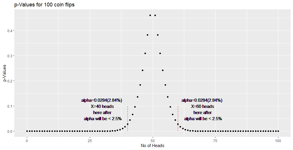
For the above binomial distribution,

• Null hypothesis H₀ = 50 heads
• At 5% significance level (α) we get 95% confidence (1-α)
• We reject H₀, when we get <40 heads (2.5%) or >60 heads (2.5%).
• i.e., 95% of the time we correctly conclude that the coin is indeed fair
• i.e., 95% of the time we correctly accept H₀
• i.e., 5% of the time we erroneously conclude that the coin is unfair.
• i.e., 5% of the time we erroneously reject H₀. This leads to Type-I error. (Fail to accept H₀ when it is true)