HVAC duct air pressure loss

This document describes the method of calculating ventilation air or conditioned air pressure loss across a rectangular duct with the help of the Darcy Weisbach equation and Colebrook equation or Moody’s chart.

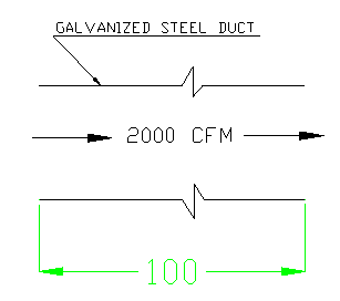
Let us assume a straight duct of 12” Height x 18” Width x 100” Length, through which 2000 cfm of air is passing. Refer to the below image for details.

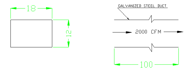
We can define the below values from the details given in the above image

Find below assumed air constants

Find below assumed material constants

Find below calculated values

Renoyld number (Re):

$R_e = \dfrac{d_h * v * \rho} {\mu}$

$=\dfrac{(14.4/12) * (1333*60) * 0.0751} {0.04462}$

$= 161578$

Friction loss co-efficient (Lambda):

If,

$R_e$ < 2300 then the flow is Laminar
$R_e$ > 2300 and $R_e$ < 4000 then the flow is transient
$R_e$ > 4000 then the flow is Turbulent

For Laminar flow

Friction loss co-efficient
$\lambda = \dfrac {64} {R_e}$

For Turbulent flow

We have to use Moody’s chart or Colebrooke equation.

Moody’s chart:

$\lambda$ is a function of $R_e$ and $\dfrac {\epsilon} {d_h}$

$\lambda = f (R_e, \dfrac {\epsilon} {d_h})$

$\dfrac {\epsilon} {d_h} = \dfrac{0.0036} {14.4} = 0.00025$

From Moody’s chart you can find the below value

$\lambda = 0.0144$ @ {$R_e = 161578$ and $\dfrac {\epsilon} {d_h} = 0.00025$}

Colebrooke equation:

$\dfrac{1} {\sqrt{\lambda}}= -2 * \log(\dfrac{2.51} {R_e * \sqrt{\lambda}} + \dfrac{k}{dh * 3.72})$

Slove the above equation by trial and error method (iterate) using different values for λ.

Resolved λ = 0.0179

Pressure loss using Darcy Weisbach equation:

$\Delta P = \lambda * \dfrac{l}{d_h} * \dfrac{\rho*v^2}{2}$

$= 0.0179 * \dfrac{100}{14.4} * \dfrac{0.00237*1333^2}{2}$

$= 0.0727 \dfrac {lb_f}{ft^2}$

$= 0.014$ $inch$ $of$ $H_2 O$