Uniform distribution

by theDataTalks . 26 Apr 2020

Uniform-distribution:

A distribution, where each outcome has probability of equally, likely chances and they are impossible beyond a range.

These are discrete uniform distribution:

Consider a draw of cards(suit) from a deck of playing cards, each suit (clubs, hearts, diamonds & spades) will have a probability of equally, likely chances of 1/4.
The number of values are finite for each suit. We can not get other than 2 to 10, ace, jack, queen & king.

Consider a roll of a die having 6 faces (1,2,3,4,5 & 6), each face will have a probability of equally, likely chances of 1/6.
The number of values are finite viz., 1,2,3,4,5 & 6. We can not get 1.2, 8, 2.6 or some other value.

The probability mass function(PMF), which gives the probability of x

$\begin{array}{c} p(x) \geq 0 AND \sum_{i=1}^n p(x) =1\\\ p(x) = p(X=x) \end{array}$

The below images are explaining the PMF of single fair dice & two fair dice.

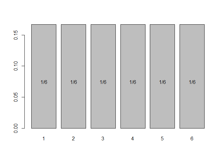
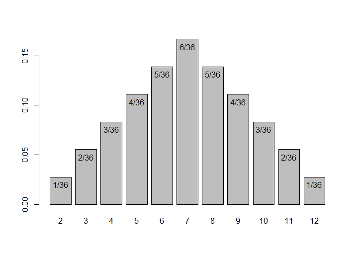
Here the dice are fair and they are not biased.

Notice the change in the shape of the graph. When the number of dice increases, the curve get closer to bell shape and the curve widens.
It always approximates to normal distribution.

Examples:

Single fair dice - Probability to get 3 is 1/6
Single fair dice - Probablity to get greater than or equal to 3 & less than are equal to 5 is 1/6+1/6+1/6 = 3/6 = 1/2
Two fair dice - Probability to get 2 is 1/36
Two fair dice - Probablity to get greater than or equal to 3 & less than are equal to 5 is 3/36+6/36+10/36 = 19/36

The cumulative distribution function(CDF), which gives the probability that the variable less than or equal to the value x

$\begin{array}{c} F(x) = p(X \leq x)\\\\ = \sum_{x_i \leq x} p(x_i)\\\\ = p(x_1)+p(x_2)+p(x_3)+...+p(x) \end{array}$

The below images are explaining the CDF of single fair dice & two fair dice.

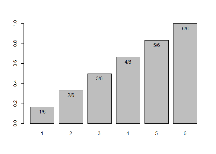
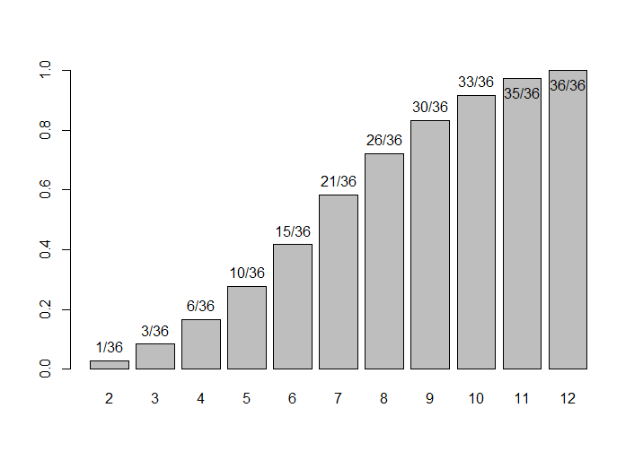
Here the dices are fair & they are not biased.

Examples:

Single fair dice - Probability to get less than 3 is 1/6+1/6+1/6 = 3/6 = 1/2
Two fair dice - Probablity to get less 3 is 1/36+3/36 = 4/36 = 1/9

If X is a discrete random variable then the Population Mean

$\begin{array}{c} \mu = E[X] = \sum {x * p(x)} \end{array}$

If X is a discrete random variable then the Population variance

$\begin{array}{c} \sigma^2 = E[(X-\mu)^2] = \sum {(x-\mu)^2 * p(x)}\\\\ \text{The same can be written as }\\\\ \sigma^2 = E[X^2]-\mu^2 = \sum{x^2*p(x)-\mu^2} \end{array}$

Examples:

Mean & variance of a single dice are

Mean = (1 * 1/6) + (2 * 1/6) + (3 * 1/6) + (4 * 1/6) + (5 * 1/6) + (6 * 1/6) = 21/6 = 3.5

The same can be calculated using below formula
Mean = (n + n * 6)/2
Here, 6 - is the number of faces on a dice & n - is the number of dice
So, Mean = (1+1*6)/2 = 7/2 = 3.5

Variance = [(1-3.5)^2 * 1/6 + (2-3.5)^2 * 1/6 + (3-3.5)^2 * 1/6 + (4-3.5)^2 * 1/6 + (5-3.5)^2 * 1/6 + (6-3.5)^2 * 1/6
= 70/24 = 35/12 = 2.91

The same can be calculated using below formula
Mean = n * 35/12
n - is the number of dice
So, Variance = 1* 35/12 = 2.91

Mean & variance of a 2 & 3 dice are

For, 2 Dice
Mean = (2+2*6)/ = 14/2 = 7
Variance = 2 * 35/12 = 5.83

For, 3 Dice
Mean = (3+3*6)/ = 21/2 = 10.5
Variance = 3 * 35/12 = 8.75

These are continious uniform distribution:

Consider a random variable(a random number generation) between any two numbers. It can take any real numbers with in the range.
The number of values are finite with in the range and they are continuous.

These variables will have probability of equally likely chances with in a range at the same time the chances are impossible beyond the specified range.

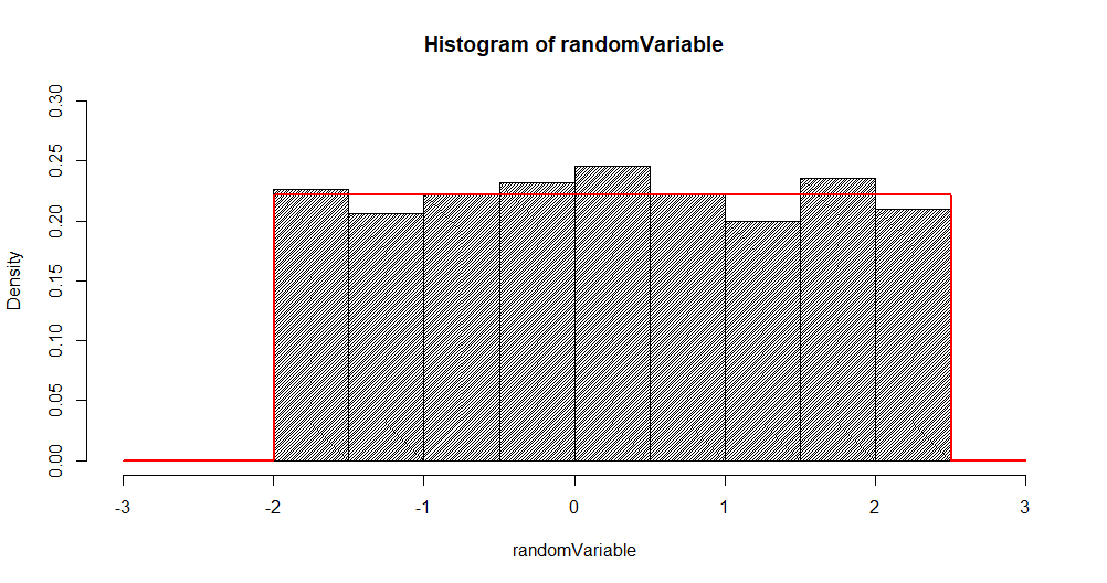
The below image represents a continuous uniform distribution and it is generated using the below specified R-command

randomVariable <- runif(1000, min = -2, max = 2.5)  
hist(randomVariable, density = 50, freq = FALSE, xlim = c(-3,3), ylim = c(0, 0.3))  
curve(dunif(x, min = -2, max =2.5), from = -3, to = 3, n=1000, add = TRUE, col = "red", lwd=2)

1000 random numbers were generated between -2 & 2.5.
Minimum value ‘a’ = -2 & maximum value ‘b’ = 2.5.

Here,

$\begin{array}{c} Density = f(x) = {1 \over (b-a)} \\\\ Mean = \mu = {(b+a) \over 2} \\\\ Variance = \sigma^2 = {(b-a)^2 \over 12} \end{array}$