Navier Stokes Equation

Newtons second law states that

$F = ma$

$F = m \times \frac{dv}{dt}$

If the mass is changing with time

$F = \frac{d(mv)}{dt}$

The above equation can be written for three dimensions

$f_x = \frac{d(mv_x)}{dt}; f_y = \frac{d(mv_y)}{dt}; f_z = \frac{d(mv_z)}{dt}$

The above three terms can be combined and written as

$F = \frac{D}{Dt} (mV)$

Divide this equation by volume

$f = \frac{D}{Dt} (\rho U)$

Consider a specific cell (finite volume) in a fluid domain (example: Nozzle flow), who’s property under goes following changes

• changing its location with respect time ($\frac{\partial}{\partial t}$)
• momentum change in spacial location ($\frac{\partial}{\partial x} u_x + \frac{\partial}{\partial y} u_y + \frac{\partial}{\partial z} u_z$)

So total change in any property with respect to time is

$\frac{D}{Dt} = \frac{\partial}{\partial t} + \frac{\partial}{\partial x} u_x + \frac{\partial}{\partial y} u_y + \frac{\partial}{\partial z} u_z$

Using dot product rule

$\frac{D}{Dt} = \frac{\partial}{\partial t} + \nabla . U$

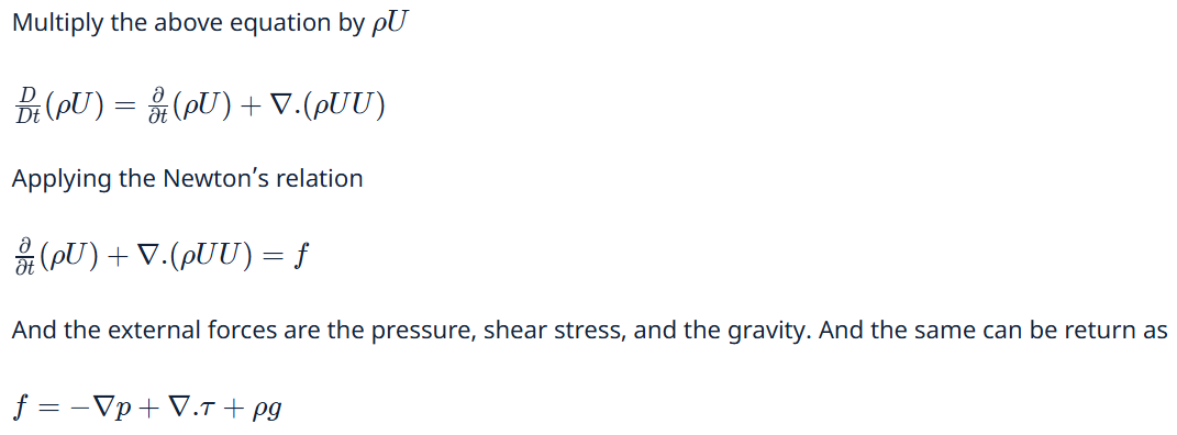
Multiply the above equation by $\rho U$

$\frac{D}{Dt} (\rho U) = \frac{\partial}{\partial t} (\rho U) + \nabla . (\rho U U)$

Applying the Newton’s relation

$\frac{\partial}{\partial t} (\rho U) + \nabla . (\rho U U) = f$

And the external forces are the pressure, shear stress, and the gravity. And the same can be return as

$f = -\nabla p + \nabla . \tau + \rho g$